While on vacation in a mysterious city, you take a wrong turn down a dark alley and are approached by two unusually generous street hustlers.

The first offers to play a simple coin game. After you wager any sum of money $M$, he’ll flip a fair coin. If it comes up $heads$, he’ll pay you $M$, but if it’s $tails$, you’ll owe him $\frac{M}{2}$.

Before you have a chance to accept, the second hustler proposes a slight variation on the same game. You’ll still wager $M$, but instead he’ll flip a coin for each dollar of your bet. Every time it lands on heads, you win $\$1.00$, but each tails will cost you $\$0.50$.

Which game should you play?

Expected value
Variance and downside risk
Real-world examples
Conclusion

Expected value

At first glance these games might look identical, and from the perspective of expected value, they are. The payout for the first game ($G_1$) is calculated by:

\[E_1=P_{heads}\times{M} - P_{tails}\times\frac{M}{2}\]

Assuming a fair coin, and a $\$10$ wager, you have an equal chance of winning $\$10$ or losing $\$5$, for an average payout of $\$2.50$. Pretty good odds! And although the second game ($G_2$) takes a little longer to play, it’s clear that the expected value is the same:

\[E_2=\sum_{n=1}^{M} (P_{heads}\times{\$1.00} - P_{tails}\times{\$0.50})\]

For each flip of the coin, you have an equal chance of winning $\$1.00$ or losing $\$0.50$, for an average of $\$0.25$. For a $\$10$ wager, with 10 corresponding flips, you’d still expect to win $\$2.50$.

But despite the identical expected payout, there is a good reason to prefer one game over the other.

Variance and downside risk

Imagine you choose to play $G_1$, and now have to decide how much to wager. You know, from the expected value calculations above, that you’ll get a $25\%$ payout, on average. Clearly you should wager more than $\$10$, but is there any limit to how much you should be willing to bet?

Perhaps you’ve already identified a problem. While you have a $50\%$ chance of doubling your money, you also have a $50\%$ chance of losing half of it; a risky proposition! In order to visualize this risk, we can plot the probability and payoff associated with each possible outcome:

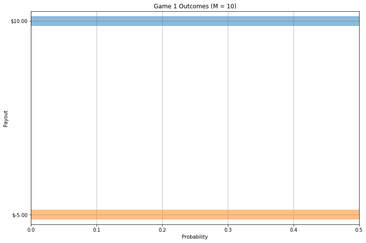
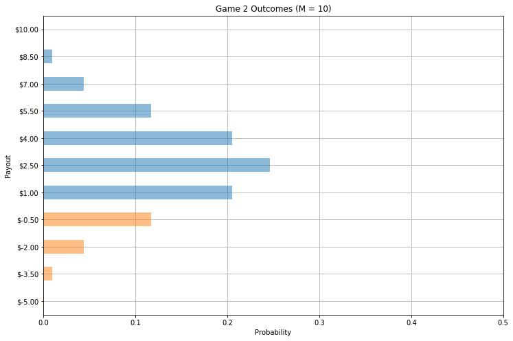
As the bar chart above shows, with a bet of $M=\$10$ there are two equal probability outcomes for $G_1$; one (blue) in which you win $\$10$, and the other (orange) where you lose $\$5$. Looking at the outcomes for $G_2$, however, something is clearly different:

Even without analyzing the math, it’s obvious that, while in $G_1$ $50\%$ of the outcomes were negative (orange), in $G_2$ you only expect to actually lose money on a handful of bets (about $17\%$).

A more formal name for the bars in orange is downside risk, a term that represents the probability of a negative outcome for a particular strategy. This is closely related to the variance, or spread, of the underlying probability distribution, since larger variance means a longer tail, and therefore more area in the negative region.

In $G_1$, the probabilities are maximally spread, leading to the outcome with the largest downside risk. With $G_2$, however, each additional dollar you bet is another coin flip, and the more coins get flipped, the more likely you are to get a result close to the expected value (since each flip is independent of the previous one). You can test this yourself!

Real-world examples

In summary, picking $G_2$ has the advantage of significantly reducing the risk relative to $G_1$ without sacrificing any expected value. But is this relevant outside of hypothetical street games in dark alleys of mysterious cities?

Finance

The obvious example of downside risk in the real world is in finance, the industry responsible for coining the term. When analyzing a portfolio of stocks, investors often care about more than just the expected return of the individual assets. Young adults, with 30+ year careers ahead of them, can afford to prefer relatively risky investments, since they are playing $G_2$, and each additional year represents another flip of the coin pushing their returns towards the expected value in the long run. Workers approaching retirement, however, are in $G_1$, and can’t afford to take risks with their accumulated capital, even at the expense of losing out on higher returns.

One tool for managing portfolio risk is (Post-)Modern Portfolio Theory, which considers both the expected return and covariance of each of the individual stocks. Stocks that are highly covariant, such as companies within the same sector, tend to move up and down together as market conditions change. Investing with a portfolio full of highly covariant stocks is a single flip game, similar to $G_1$ above, and may be just as risky as owning a single stock in that sector.

A better strategy is to create a balanced portfolio, full of stocks with high expected returns but uncorrelated variance. That way if an individual stock or whole sector loses value, it’s unlikely to have a significant impact on overall returns, similar to losing a single flip in $G_2$.

Effective Altruism

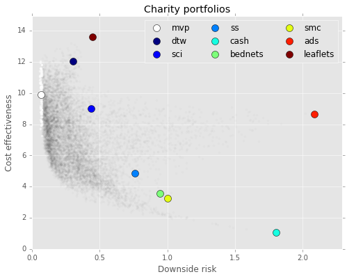
The same is likely true of charities, as I’ve talked about in a series of previous posts about stochastic altruism. As with stocks, even when trying to maximize expected value (or good deeds per dollar donated, in this case), it can still be beneficial to distribute donations among several charities with uncorrelated variance. A balanced portfolio of charities can provide similar altruistic returns with significantly reduced downside risk.

And thinking about Effective Altruism (EA) in the context of $G_1$ vs. $G_2$ has other implications as well.

In another post I summarized David Roodman’s research on the “Worm Wars”, the dramatized name for the debate within medical literature on the efficacy of deworming interventions. Though I won’t completely rehash it here, my (non-expert) understanding is that the argument turns on how much credence should be given to series of studies showing that childhood deworming medication leads to an increase in consumption (and presumably well-being) later in life.

A simplified view of the problem might be that we either live in a world in which deworming works or we do not. In the former, most children would benefit from deworming medication to some degree, but in the latter, all of our money is wasted and would be better donated elsewhere. This scenario is reminiscent of $G_1$; a single flip problem with high downside risk.

And not all EA interventions share this particular issue. GiveDirectly, for example, distributes money collected from donors to poor families in Kenya and Uganda. After running several randomized control trials on this intervention, it’s clear that this is a boon for most recipients, with only a handful reporting any negative outcomes. Generally, interventions like this are more similar to $G_2$, with a “flip” for each recipient, and are less prone to systemic downside risk.

Hockey and upside risk

By slightly reframing the concept of risk, we can apply a similar model to decisions made at the end of hockey games. If a team is losing by a narrow margin with only a few minutes remaining, a common strategy is to replace the goalie with an extra attacker. Although this increases the risk of allowing the opponent to score on the now-empty net, it also makes it more likely that them team will score the tying goal. And since the margin of victory is (mostly) irrelevant in hockey standings, it sometimes represents a good tradeoff:

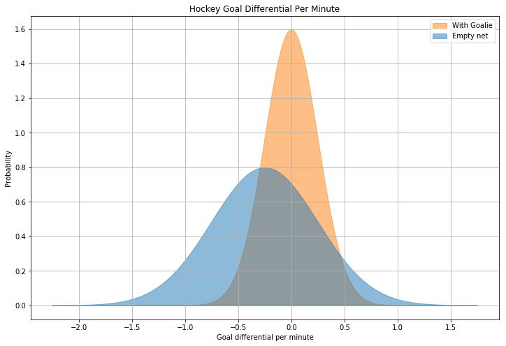
Whereas we were previously trying to minimize downside risk by choosing $G_2$ over $G_1$, in the case of the losing hockey team, it’s advantageous to increase the variance (even at the cost of a larger expected losing margin) in order to capture some “upside” risk. As a demonstration, consider the following graph, which shows (made up but plausible) probability density functions for the expected goal differential per minute, with and without a goalie:

The two curves above are normal distributions, $\mathcal{N_1}(0.0,\, 0.0625)$ (orange, with a goalie) and $\mathcal{N_2}(-0.25,\, 0.25)$ (blue, without). When the goalie is pulled, we expect the losing team to fall even further behind, with the goal differential increasing by $0.25$ per minute on average. However, with the goalie in the game, it’s extremely unlikely that they will score the tying goal, with that probability represented by the area under the orange curve at $X \geq 1$. Even though the blue distribution has a lower expected value, it also has more area under this same section of the curve, representing a higher chance of scoring the tying goal. In fact, if this data were accurate, it would predict that the losing team should pull their goalie with four minutes remaining in the game, not far from the apparently optimal strategy of approximately three minutes.

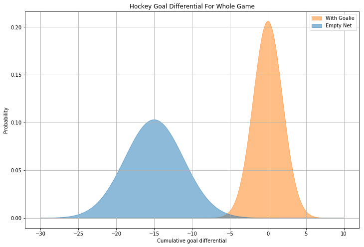
And why not play without a goalie for the full sixty minutes? As it turns out, pulling the goalie can be viewed as an attempt to move the endgame from $G_2$ to $G_1$ in order to capture the “upside” risk of a low probability outcome. The longer the team plays without a goalie, however, the more minutes they accumulate with the new probability distribution, and the more the game resembles $G_2$ again, with the accumulated expected value outweighing the uncorrelated variance:

\[m\times{\mathcal{N}(\mu,\, \sigma^{2})} = \mathcal{N}(m\times{\mu},\, m\times{\sigma^{2}})\]

Given the assumptions above, a hockey team playing without a goalie for the whole game could expect to lose by more than 15 goals!

Conclusion

In writing this post, I was gratified to find that some of my disparate thoughts from the past few years can be derived in terms of the same simple thought experiment. The issues with expected value are not unknown, even within the EA community, but statistics are notoriously counterintuitive, and concepts like uncorrelated variance and downside risk seem correspondingly undervalued in popular discourse.

If you take one thing away from this post, try conceptualizing problems not just by their expected value, but also through the lens of $G_1$ and $G_2$ (even when not in dark alleys in mysterious cities). For “games” with similar payouts, prefer those that resemble $G_2$. When constructing portfolios of things like stocks or charities, be wary of accidentally playing $G_1$ by selecting assets with highly correlated variance. And if you’re down big with only a few minutes to go, try to change the game back to $G_1$, especially if you’re playing hockey.